Synchronized robot motion: how OLP makes multi-robot programming manageable
Multi-robot cells can weld, handle, and reposition large parts in ways one robot cannot. Offline programming gives engineers one place to program the complete system and find problems before commissioning.
A welding robot is halfway along a seam when the positioner starts to turn. The seam moves, the torch follows, and both sets of axes have to stay in step. Now add a second welding robot on the other side of the part. A program edit that looks harmless for one robot can put the other robot in its path.
These setups can improve access and keep the process moving. They also make programming much harder. Every moving axis changes the geometry for something else. A small path edit can affect clearance, timing, and the motion of another robot.
Some synchronized controllers let one teach pendant hold the programs for all robots in the system. That helps centralize control, but it doesn’t remove the manual work. The programmer still has to activate the correct robot or mechanical unit and confirm which machines can move. Selecting the wrong unit or leaving another machine active can cause a serious collision.
Multi-robot offline programming (OLP) moves this work into a shared 3D environment. Engineers can program the complete cell, test how motions interact, and generate controller-specific robot code before commissioning. On-site work remains, but commissioning starts with a calibrated model and tested programs.
What synchronized robot motion actually means
Teams often use coordinated and synchronized motion interchangeably. Robot manufacturers also use their own terms, so one definition doesn’t map cleanly to every controller.
Here, coordinated operation means that two or more devices follow a planned relationship. They might exchange signals, wait at defined points, or run timed paths to avoid a conflict.
Synchronized motion is tighter. Multiple mechanical units move as one controller-managed motion system. The synchronization may be time-based, distance-based, or based on another relationship supported by the robot configuration and communication setup. A robot can follow a target defined relative to a workpiece that is moving on another robot or an external axis.
Consider arc welding with a rotating positioner. If the positioner turns, stops, and then lets the robot weld a static seam, the sequence is coordinated. If the positioner keeps rotating while the torch follows the seam, the axes move in a synchronized relationship. The robot’s target is no longer fixed in the world coordinate system.
Common configurations include:
- One robot and a rotary or tilt-rotate positioner
- Two or more robots working on the same workpiece
- One robot holding a part while another welds, cuts, grinds, coats, or inspects it
- A robot mounted on a floor track or gantry
- Several arms sharing a restricted workspace
The controller and its software options determine which relationships the physical system can execute. OLP can model a multi-brand line and coordinate program logic between cells. It cannot make incompatible controllers perform tightly coupled, real-time motion. This normally requires supported robots and mechanical units within the same controller ecosystem.
Why pendant programming gets difficult in multi-robot cells
Teach pendants work well for checking a point or making a small adjustment. They don’t give the programmer the same view of the complete system as a 3D simulation.
Even when one pendant manages several robots, the programmer must track the active robot, mechanical units, program task, and machines allowed to move. A safe move for robot A doesn’t prove that robot B will be clear when both run together. Testing this on the shop floor means moving real equipment while watching several systems.
Coordinate systems add another challenge. A path may be defined relative to the workpiece, but that workpiece can move on a positioner or in another robot’s gripper. Tool center points, work object frames, base frames, and external-axis positions all have to agree.
Changes spread through the cell. Move one weld to improve access and you may create a collision on the other side. A new positioner angle might solve one reach problem while pushing another robot toward a joint limit.
The physical cell is an expensive place to sort this out. On-site programming occupies equipment and may stop production. Each unresolved problem also takes time from commissioning.
How multi-robot offline programming works
OLP puts every relevant moving device in one model. A practical workflow has six steps.
1. Build the complete cell
Import the workpiece and fixture geometry. Add the robots, tools, positioners, tracks, tables, and safety equipment. Define their kinematic relationships.
Geometry alone isn’t enough. The virtual cell has to match the physical one. During robot cell calibration, engineers measure the real robots, tools, fixtures, and external axes. They then use those measurements to align the model.
2. Define frames and motion relationships
Set the tool and workpiece frames. Then define which device carries the workpiece and which robot follows it. In a synchronized welding setup, the workpiece coordinate system moves with the positioner or handling robot. The welding robot maintains the required path and torch angle relative to the part.
The exact relationship depends on the controller. It may follow time, distance, a leader-follower setup, or another controller-specific method. The virtual setup needs to reflect the method that the real controller supports.
3. Program every device in the same environment
Create process paths from the product geometry. Then add approach, departure, and transfer motions. Automated programming and path-solving tools can speed up this work and resolve some collisions, joint-limit problems, and reachability errors within an individual robot program.
The engineer can see every program while planning access and handoffs. The sequence still needs an engineer who understands the process.
4. Add synchronization and signal logic
Define start conditions, waits, handshakes, shared-zone access, and controller-specific synchronization points. Use continuous synchronization only where the process needs it. Many operations simply need the robots to take turns reliably through signals and waits.
5. Simulate and correct the system
Run each path on its own and then run the complete sequence. Check collisions, near misses, reach, joint limits, singularities, process orientation, and the order of operations. Test likely changes too, such as a revised fixture position or weld sequence.
6. Generate controller-specific programs
Run the correct post-processor for each robot and controller. Visual Components converts the programmed operations into the required controller language. The exact output depends on the robot brand, controller generation, installed technology packages, and cell configuration.
Generated code still needs controlled deployment. Back up the controller, confirm the configuration and frames, test at reduced speed, and complete physical acceptance checks.
What simulation can validate before deployment
A multi-robot model should answer practical questions before the real cell runs.
| Check | What the engineer learns |
| Reachability | Whether every process and transfer position is reachable across the full range of external-axis motion |
| Collision clearance | Whether robots, tools, parts, fixtures, positioners, and other moving equipment stay clear throughout the sequence |
| Joint limits and singularities | Whether a valid Cartesian path drives an arm into an unstable or impossible joint configuration |
| Process orientation | Whether the torch, gun, cutter, or tool maintains the required angle while the workpiece moves |
| Synchronization logic | Whether robots wait, exchange signals, and enter shared zones in the intended order |
| Cycle time | Whether the planned sequence can support the target output and where robots spend time waiting |
Cycle-time results need context. Visual Components uses a generic motion controller for the standard estimate. This helps compare layouts and sequences, but it won’t reproduce every brand controller to the millisecond. When exact timing is critical, engineers can connect Visual Components to supported brand-specific virtual controllers for a more detailed check.
Simulation only checks what is in the model. Poor calibration can spoil an otherwise clean result. So can the wrong payload, a missing cable package, or a fixture that doesn’t match the one on the floor.
Brand-specific synchronized motion support
The engineering workflow stays consistent across brands. The controller concepts and output do not.
ABB MultiMove
ABB MultiMove coordinates multiple robot tasks and mechanical units through an ABB controller. Visual Components supports MultiMove configurations, including coordinated and independent motion, event synchronization, and task coordination. The ABB post-processor generates RAPID output for the configured system.
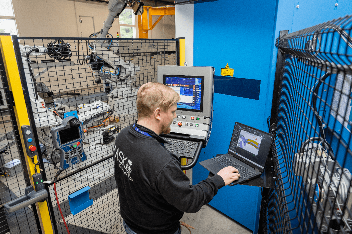
MSK Finland used this workflow for a three-robot ABB MultiMove welding cell. The team programmed the cell offline before the real system was assembled. One robot handles the jig as a workpiece positioner for two welding robots. MSK also programmed a second MultiMove system with two robots, two workpiece positioners, and a floor track.
KUKA, FANUC, and Yaskawa
KUKA, FANUC, and Yaskawa controllers use their own methods to coordinate robots and external axes. Terminology, optional software, program structure, and controller constraints differ. A FANUC coordinated-motion setup, for example, isn’t ABB MultiMove with different syntax. The same applies to KUKA and Yaskawa systems.
Visual Components supports multi-robot modeling, signal logic, external axes, and controller-specific post-processing. However, support for a brand doesn’t mean every synchronization option works the same way on every controller generation.
Before committing to a cell design, confirm the robot models, controller versions, installed software options, mechanical-unit configuration, communication setup, and required post-processors with the Visual Components OLP team. This check matters most when the application needs tightly synchronized motion. Visual Components can model signal-coordinated, multi-brand cells in one environment. Continuous synchronized motion is different: the real controller architecture sets the boundary.
Where synchronized motion creates the most value
Robot and positioner welding
Continuous positioner motion can keep a long weld in a favorable orientation and within the robot’s reach. This only works when the seam, workpiece frame, torch angle, robot arm, and positioner motion stay aligned throughout the weld.
Two-robot welding
Two arms can work on different sides of a large structure, but their safe envelopes may overlap. Simulation helps engineers plan simultaneous work, reserve shared zones, and check that one robot’s torch or cable arrangement doesn’t interfere with the other.
Coordinated handling and processing
One robot can present or reposition a part while another grinds, coats, cuts, or inspects it. This may reduce the need for dedicated fixtures, though it makes calibration and frame management more demanding. The guide to robot programming for industrial processes explains surface coverage, tool orientation, and painting paths in more detail.
Tracks, gantries, and large workpieces
External axes extend reach, but they add more possible configurations for every target. OLP lets the engineer evaluate the combined motion range instead of checking the arm and track separately.
Program the system, not one robot at a time
Multi-robot cells put a lot of motion into a small space. Reach, clearance, timing, frames, and controller logic are connected. Change one and the others may change with it.
OLP gives engineers a clear view of those effects before production equipment starts moving. They can program motion in context, run the complete sequence, and generate code for each configured controller.
Calibration, controller knowledge, and on-site testing still matter. But the first full run shouldn’t be the first time anyone has seen the robots move together.
Explore Visual Components Robotics OLP or book a demo.
Frequently asked questions
Programming with a teach pendant becomes difficult because the programmer must keep track of multiple robots, mechanical units, active tasks, and which machines are allowed to move. A path that appears safe for one robot may create a collision risk for another. Additionally, moving workpieces, coordinate systems, and external axes make it harder to understand the impact of changes across the entire cell.
OLP allows engineers to program all robots, positioners, tracks, and tools within a shared 3D environment. They can test interactions, simulate motions, detect collisions, verify synchronization, and generate controller-specific robot code before commissioning. This reduces risks, shortens on-site programming time, and helps identify issues before production equipment is used.
Simulation can validate reachability, collision clearance, joint limits, singularities, process orientation, synchronization logic, and cycle times. By testing these factors in a virtual model, engineers can identify potential problems and optimise the system before running the real cell.

Further reading

Mike Strahlman on what comes next for Visual Components
As the new CEO of Visual Components, Mike Strahlman shares his vision for the future of manufacturing simulation, digital twins, and automation planning. In this interview, he explains why factories...
Cost per weld: how to compare robot programming software as production scales
Calculate robot programming software cost per weld and compare license, subscription, and weld-credit pricing as parts and variants scale.
Introducing FactoryLens: turn factory simulations into realistic customer experiences
Visual Components launches FactoryLens, extending its collaboration with NVIDIA for industrial digital twins. FactoryLens helps system integrators and machine builders present Visual Components simulations with realistic materials, lighting, and shadows,...